Qiskit implementation

In this section, we'll take a look at some Qiskit implementations of the concepts introduced in this lesson. If you wish to run these implementations yourself, which is strongly encouraged, consult the Install Qiskit page in the IBM Quantum Documentation for details on how to set up Qiskit.

It should be understood that Qiskit is under continual development, and is principally focused on maximizing the performance of the quantum computers it is used to operate, which themselves continue to evolve. As a result, Qiskit is subject to changes that may occasionally lead to code deprecation. With this in mind, we'll always execute the following commands prior to presenting examples of Qiskit code in this course, so that it is clear which version of Qiskit has been used. Starting with Qiskit v1.0, this is a simple way to see what version of Qiskit is currently installed.

from qiskit import __version__
 
print(__version__)

Output:

2.1.1

Vectors and matrices in Python

Qiskit uses the Python programming language, so before discussing Qiskit specifically, it may be helpful to very briefly discuss matrix and vector computations in Python.

In Python, matrix and vector computations can be performed using the array class from the NumPy library, which provides functionality for many numerical and scientific computations. The following code loads this library, defines two column vectors, ket0 and ket1, corresponding to the qubit state vectors $\vert 0\rangle$ and $\vert 1\rangle,$ and then prints their average.

import numpy as np
 
ket0 = np.array([[1], [0]])
ket1 = np.array([[0], [1]])
 
print(ket0 / 2 + ket1 / 2)

Output:

[[0.5]
 [0.5]]

We can also use array to create matrices that can represent operations.

M1 = np.array([[1, 1], [0, 0]])
M2 = np.array([[1, 0], [0, 1]])
M = M1 / 2 + M2 / 2
print(M)

Output:

[[1.  0.5]
 [0.  0.5]]

Please note that all code appearing within a given lesson in this course is expected to be run sequentially. Therefore, we don't need to import NumPy again here, because it has already been imported.

Matrix multiplication, including matrix-vector multiplication as a special case, can be performed using the matmul function from NumPy.

print(np.matmul(M1, ket1))
print(np.matmul(M1, M2))
print(np.matmul(M, M))

Output:

[[1]
 [0]]
[[1 1]
 [0 0]]
[[1.   0.75]
 [0.   0.25]]

This output formatting leaves something to be desired, visually speaking. One solution, for situations that demand something prettier, is to use thearray_to_latex function in Qiskit, from the qiskit.visualization module. Note that, in the code that follow, we're using Python's generic display function. In contrast, the specific behavior of print may depending on what is printed, such as it does for arrays defined by NumPy.

from qiskit.visualization import array_to_latex
 
display(array_to_latex(np.matmul(M1, ket1)))
display(array_to_latex(np.matmul(M1, M2)))
display(array_to_latex(np.matmul(M, M)))

Output:

States, measurements, and operations

Qiskit includes several classes that allow for states, measurements, and operations to be created and manipulated — so there is no need to program everything required to simulate quantum states, measurements, and operations in Python. Some examples to help you to get started are included below.

Define and display state vectors

TheStatevector class in Qiskit provides functionality for defining and manipulating quantum state vectors. In the code that follows, the Statevector class is imported and a few vectors are defined. (We're also importing the sqrt function from the NumPy library to compute a square root. This function could, alternatively, be called as np.sqrt provided that NumPy has already been imported, as it has above; this is merely a different way to import and use this specific function alone.)

from qiskit.quantum_info import Statevector
from numpy import sqrt
 
u = Statevector([1 / sqrt(2), 1 / sqrt(2)])
v = Statevector([(1 + 2.0j) / 3, -2 / 3])
w = Statevector([1 / 3, 2 / 3])

The Statevector class includes a draw method for displaying state vectors in a variety of ways, including text for plain text, latex for rendered LaTeX, and latex_source for LaTeX code, which can be handy for cutting and pasting into documents. (Use print rather than display to show LaTeX code for best results.)

display(u.draw("text"))
display(u.draw("latex"))
print(u.draw("latex_source"))

Output:

[0.70710678+0.j,0.70710678+0.j]

$\frac{\sqrt{2}}{2} |0\rangle+\frac{\sqrt{2}}{2} |1\rangle$

\frac{\sqrt{2}}{2} |0\rangle+\frac{\sqrt{2}}{2} |1\rangle

The Statevector class also includes the is_valid method, which checks to see if a given vector is a valid quantum state vector (in other words, that it has Euclidean norm equal to 1):

display(u.is_valid())
display(w.is_valid())

Output:

True

False

Simulating measurements using Statevector

Next we will see one way that measurements of quantum states can be simulated in Qiskit, using the measure method from the Statevector class. Let's use the same qubit state vector v defined previously.

display(v.draw("latex"))

Output:

$(\frac{1}{3} + \frac{2 i}{3}) |0\rangle- \frac{2}{3} |1\rangle$

Running the measure method simulates a standard basis measurement. It returns the outcome of that measurement, plus the new quantum state vector of the system after the measurement. (Here we're using Python's print function with an f prefix for formatted printing with embedded expressions.)

outcome, state = v.measure()
print(f"Measured: {outcome}\nPost-measurement state:")
display(state.draw("latex"))

Output:

Measured: 1
Post-measurement state:

$- |1\rangle$

Measurement outcomes are probabilistic, so this method can return different results when run multiple times. For the particular example of the vector v defined above, the measure method defines the quantum state vector after the measurement takes place to be

(rather than $\vert 0\rangle$) or

(rather than $\vert 1\rangle$), depending on the measurement outcome. In both cases, the alternatives to $\vert 0\rangle$ and $\vert 1\rangle$ are, in fact, equivalent to these state vectors; they are said to to equivalent up to a global phase because one is equal to the other multiplied by a complex number on the unit circle. This issue is discussed in greater detail in the Quantum circuits lesson, and can safely be ignored for now.

Statevector will throw an error if the measure method is applied to an invalid quantum state vector.

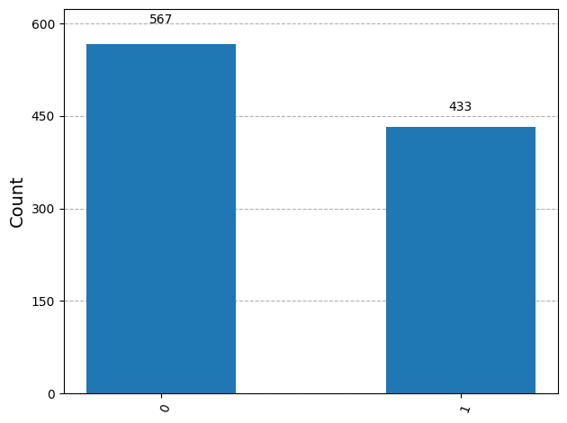
Statevector also comes with a sample_counts method that allows for the simulation of any number of measurements on the system, each time starting with a fresh copy of the state. For example, the following code shows the outcome of measuring the vector v $1000$ times, which (with high probability) results in the outcome $0$ approximately $5$ out of every $9$ times (or about $556$ of the $1000$ trials) and the outcome $1$ approximately $4$ out of every $9$ times (or about $444$ out of the $1000$ trials). The code that follows also demonstrates the plot_histogram function from the qiskit.visualization module for visualizing the results.

from qiskit.visualization import plot_histogram
 
statistics = v.sample_counts(1000)
plot_histogram(statistics)

Output:

Running this code on your own multiple times, with different numbers of samples in place of $1000,$ may be helpful for developing some intuition for how the number of trials influences the number of times each outcome appears. With more and more samples, the fraction of samples for each possibility is likely to get closer and closer to the corresponding probability. This phenomenon, more generally speaking, is known as the law of large numbers in probability theory.

Perform operations with Operator and Statevector

Unitary operations can be defined in Qiskit using the Operator class, as in the example that follows. This class includes a draw method with similar arguments to Statevector. Note that the latex option produces results equivalent to array_from_latex.

from qiskit.quantum_info import Operator
 
Y = Operator([[0, -1.0j], [1.0j, 0]])
H = Operator([[1 / sqrt(2), 1 / sqrt(2)], [1 / sqrt(2), -1 / sqrt(2)]])
S = Operator([[1, 0], [0, 1.0j]])
T = Operator([[1, 0], [0, (1 + 1.0j) / sqrt(2)]])
 
display(T.draw("latex"))

Output:

We can apply a unitary operation to a state vector using the evolve method.

v = Statevector([1, 0])
 
v = v.evolve(H)
v = v.evolve(T)
v = v.evolve(H)
v = v.evolve(S)
v = v.evolve(Y)
 
display(v.draw("latex"))

Output:

$(0.1464466094 - 0.3535533906 i) |0\rangle+(-0.3535533906 + 0.8535533906 i) |1\rangle$

A preview of quantum circuits

Quantum circuits won't be formally introduced until the Quantum circuits lesson, which is the third lesson in this course, but we can nevertheless experiment with composing qubit unitary operations using theQuantumCircuit class in Qiskit. In particular, we may define a quantum circuit (which, in this case, will simply be a sequence of unitary operations performed on a single qubit) as follows.

from qiskit import QuantumCircuit
 
circuit = QuantumCircuit(1)
 
circuit.h(0)
circuit.t(0)
circuit.h(0)
circuit.s(0)
circuit.y(0)
 
display(circuit.draw(output="mpl"))

Output:

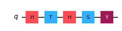
Here we're using the draw method from the QuantumCircuit class with the mpl renderer (short for Matplotlib, a Python visualization library). This is the only renderer we'll use for quantum circuits in this course, but there are other options, including a text-based and a LaTeX-based renderer.

The operations are applied sequentially, starting on the left and ending on the right in the diagram. A handy way to get the unitary matrix corresponding to this circuit is to use the from_circuit method from the Operator class.

display(Operator.from_circuit(circuit).draw("latex"))

Output:

We can also initialize a starting quantum state vector and then evolve that state according to the sequence of operations described by the circuit.

ket0 = Statevector([1, 0])
v = ket0.evolve(circuit)
display(v.draw("latex"))

Output:

$(0.1464466094 - 0.3535533906 i) |0\rangle+(-0.3535533906 + 0.8535533906 i) |1\rangle$

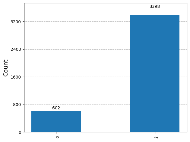
The following code simulates an experiment where the state obtained from the circuit above is measured with a standard basis measurement 4000 times (using a fresh copy of the state each time).

statistics = v.sample_counts(4000)
display(plot_histogram(statistics))

Output: